Practical 3: Free energy calculations from non-equilibrium dynamics
Bert de Groot
Contents
Introduction
In a previous tutorial we learned two methods to compute Free Energies
associated to a given thermodynamic process: the solvation Free Energy of
sodium ions in water and the folding of a peptide in water.
In the first case we used Free Energy Perturbation (FEP), that takes advantage
of the fact that Free Energy is a state function. For an equilibrium process,
the Free Energy is independent of
the path the system takes to move from state A (no sodium in water) to state B
(sodium fully solvated in water).
As the sodium-water interactions were slowly
turned on, we recorded the changes in potential energy. Integration of these
potential energy differences over the morphing path yields the Free Energy.
To study the themodynamics of peptide folding, we relied on the Boltzamn
probability distribution of themodynamic ensembles in equilibrium. The
relative population of folded and unfolded states was extracted from a
molecular dynamics simulation, which gives direct access to Free Energy differences.
So far we have used equilibrium dynamics to compute Free Energies: the
transition between states is done infinitely slow, or reasonably slow, and the
work performed/gained is equal to the Free Energy. By extracting Free Energies
from equilibrium simulations we have to make sure that the system fulfills a
Boltzmann equilibrium. In practice this means that we have to sufficiently
sample the phase space available. While this is conceptually not a problem, in
practice this poses a problem for systems with many degrees of freedom and long
relaxation times.
The Jarzynski equation
As a follow up, today we will learn that we can use non-equilibrium dynamics to
compute Free Energies. Although several new relationships for non-equilibrium thermodynamics
were found during last century, the link between the work and the Free Energy remained
as an inequality: the work is always greater or equal to the underlying equilibrium Free
Energy (  ). It was not until the very end of last century (1997-1998) that new
expressions directly relating the work and the Free Energy were found. The first one, known
as the Jarzynski equation, relates the ensemble average over an exponential distribution
of the work with the Free Energy.
). It was not until the very end of last century (1997-1998) that new
expressions directly relating the work and the Free Energy were found. The first one, known
as the Jarzynski equation, relates the ensemble average over an exponential distribution
of the work with the Free Energy.
This relationship turned out to be extremely useful, as it allows,
for example, to compute binding Free Energies of ligands by repeatedly enforcing the unbinding
and recording the work distribution.
This process can be mimicked in a computer experiment, with the advantage that the simulation
times are reduced due to the fast non-equilibrium trajectory. Nevertheless, several experiments
have to be carried out to get a reasonable estimate of the work distribution.
The Crooks theorem
Yet another non-equilibrium relationship, even more fundamental, was put forward by Crooks in
1999. The expression is grounded on microscopic reversibility, and one useful theorem derived
from it is the Transient Fluctuation Theorem (TFT).
The former relates the ratio of the work distribution for a Markovian process that moves from
state A to state B and from state B to a A with the dissipated work involved in
the transformation. Look at the wikipedia
page for more information, if you're interested.
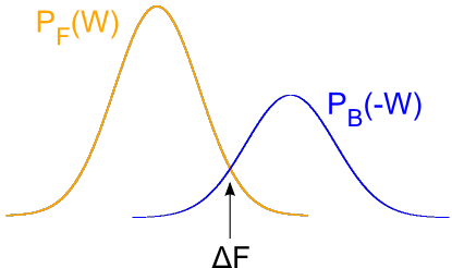
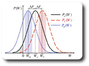
A first approach is to estimate the free energy as the work value W where both distributions overlap, PF(W) = PB(-W):
A second approach is to take the logarithm of the Crooks equation,
Then, plot the left side of this equation vs. the work, which is a straight line, and estimate the free energy from the intercept.
Today we will take advantage of these recent breakthroughs to compute Free Energies
( an equilibrium property ) from non-equilibrium processes. To illustrate the capabilities of these
relationships we will first study the solvation Free Energy of an ion in water, now by means of
several fast (non-equilibrium) Free Energy Perturbation simulations. A second application
of non-equilibrium relationships will serve us to elucidate the Free Energy profile for an ion
permeating through a peptidic ion channel.
Go back to Contents
Solvation free energy of a sodium ion in water using the Crooks theorem
This exercise uses the same simulation technique (FEP) previously introduced in these
tutorials. We learned that sufficiently long simulations were needed to obtain a converged
value for the solvation Free Energy, where the morphing parameter lambda was slowly changed
from 0 (no ion-water interactions) to 1 (all interactions switched on).
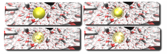
Another way of computing the solvation Free Energy would be to perform
multiple (fast) simulations. Some will drive the system from an equilibrated
state A (lambda = 0) to a final state B (lambda = 1). We will call such a
process the Forward transformation. Additionally, some will be perfomed in the
opposite direction (Reverse transformation), e.g. an equilibrated system in the
B state will be transformed into state A. By collecting the work performed in
either Forward or Reverse transformation we can obtain their respective
probability distributions. Recalling Crooks' Transient Fluctuation Theorem we
know that the point where the two probability distributions meet the dissipative
work is zero. Hence, at this point the work will equal the Free Energy.

As we saw last week, from each of the
transition simulations we get a dhdl.xvg file that contains the dH/dlambda as a function of time.
These curves can be integrated over dlambda to extract the work. As described by the Crooks theorem the intersection of the
distributions
for the forward and backward transitions are a free energy estimate.
For this week's exercise we ran many fast (10ps) simulations and obtained a dhdl.xvg file for each of them. Here you find one directory for the forward and one directory for the backward transitions.
To extract the content, use
wget http://www3.mpibpc.mpg.de/groups/de_groot/compbio/p10/400runs.tar.gz
tar -xvzf 400runs.tar.gz
We now want to plot the
distributions of the work values for the forward and backward transition to be able to use Crooks theorem.
To do so go to the directory of the forward transitions first.
To gather the work values from the dhdl.xvg files a script has been prepared. Run it
./gather_work.csh | grep -v csh > ../Work_fwd.txt
This can take a few seconds, but eventually it writes a file containing all forward work values.
To be able to use Crooks theorem we need the backward work values as well.
To collect them go to the backward directory
cd ../REV_RUN_TFT
./gather_work.csh | grep -v csh > ../Work_rev.txt
Let's see if we
computed enough values to estimate a reasonable probability distribution of the work.
If we don't have any extra information
on the distribution function, it is necessary to have an overlap between the two distributions, since Crooks' TFT
states that the work value that equals the true Free Energy is the one which has the same probability in the
forward and in the reverse distribution.
To compare the work values, we will generate histograms (or numerical estimates of unormalized probability distributions) for both work
distributions with xmgrace,
open them both directly with
cd ..
xmgrace Work_fwd.txt Work_rev.txt
To compute histograms, first of all create a new graph: Go to "edit" -> "arrange graphs" and set the "cols" value to 2.
Apply the changes and close. Now you have two graphs. To compute the histograms, go to "data" -> "transformations" and
click on "histograms". From the "source" list click now on the first (g0) and then the first "set" (go.so). As a "destination" list select the
second (g1). Now have a look at the values you have for the distribution, typically between -420 to -360. Use these numbers
as "start at" and "stop at" and something like 40 bins. The more data points,
the more bins we can use. Click in "normalize" and then press "apply" to
perform the histogram on the first data set. To obtain one for the second data set, simply select (g0.s1), under the second
"set" in the first graph in the "source" list and press "apply". In order to see the histograms, select the new graph by clicking it with the mouse and then
press the "as" (for auto scale) button on the upper left.
Question:
Based on the two adjacent histograms, what is the estimate for the free energy value and how does it compare to the
expected value of around -393 kJ/mol?
Do you think 10 simulations in each direction would have been enough to get an
reasonable estimate?
OPTIONAL: Estimation of the free energy taking the logarithm of the Crooks equation
Once you obtained the work distributions, it is possible to estimate the free energy taking the logarithm of the Crooks equation (see here). You should extract the portion of both distributions in which there is an overlap and PF(W), PB(-W) are not zero (to avoid singularities).
First recompute the histograms, and filter the overlap region (work values between -404 and -385 kJ/mol):
sort -g Work_fwd.txt | awk -f histogram.awk | awk '$1 > -404 && $1 < -385 {print $0}' > Work_fwd_over.his
sort -g Work_rev.txt | awk -f histogram.awk | awk '$1 > -404 && $1 < -385 {print $0}' > Work_rev_over.his
now collect for each non-zero count of the forward and reverse work distribution the logarithm:
paste Work_fwd_over.his Work_rev_over.his | awk '$2>0 && $4> 0 {print $1,log($2/$4)}' > W_log.txt
Then, plot ln ( PF(W) / PB(-W) ) as a function of W and do a linear regression. The slope of this curve is β = 1/KT and the intercept is -βΔ F
and in xmgrace, under Data -> Transformations, click 'Regression'.
Questions:
How much does the regression deviate from a straight line? How does the estimate of β = 1/KT compare with the input value, β = 1/(2.5 kJ/mol) , at the given temperature of 300 K? What is the estimate of the free energy? How does it compare with the previous estimations?
This is a short version of a more extended tutorial. If you are interested in running the simulations yourself you can do the first part of the original tutorial.
Go back to Contents
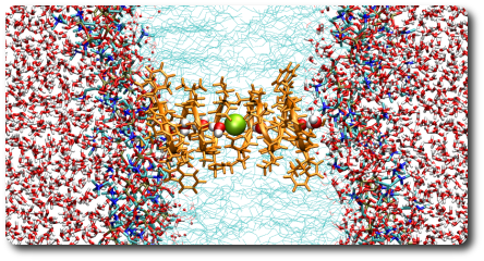
Potential of Mean Force for a potassium ion permeating an ion channel
Ion channels, located in the lipidic membrane that separates organelles or cells, allow the passage of ions
from one side of the membrane to the other. Their structure and composition is diverse, although they
share some characteristics. Gramicidin is a small peptidic ion channel of 30 aminoacids, whereas potassium
ion channels, like KcsA, are proteins with quaternary structure. Their function affects electrochemical gradients,
and thus ion channels have a fundamental role in the bioenergetics of living cells. A subtle balance of ion gradients is, for example, responsible
for the polarization-depolarization of neuron's membrane that leads to electrical signal transmission in nerve cells.
Many membrane proteins need to couple their transport mechanisms to ion gradients.
For these and many other reasons, ion channels are of great interest in biophysics and electrophysiology, as well as in medicine.
Ion channels differ from ion transporters because they do not need an external energy source to achieve their
functionality. Their activity can be gated by several means: voltage, drug binding, pressure, or simple
ion gradient.
Most ion channels present a selectivity filter to achieve specificity for certain types of ions.
These regions are usually carefully constructed to have favorable stabilizing environment for the ion they want to
permeate. Ions in solution are stabilized by the interactions with the solvation water shell, as we saw in the previous
exercise. As the ion enters the channel several interactions with solvating waters disappear,
which can not be fully compensated by the channel's partially hydrophobic interior. Since ions are charged species, this
desolvating effect is much stronger than for water, and so the ion flux is significantly lower compared to water flux.
Molecular dynamics is a very powerful tool to study the energetics of ion channels, provided a good set of parameters that
describes the interactions between channel, ions and membrane. Nevertheless, the high activation energy for ion permeation
makes direct estimation of ion flux almost impossible: the simulation time needed to observe a significant amount
of ion translocations is currently out of reach.
Luckily, rate theory provides a clear connection between the underlying energetics for ion permeation and their
rates or fluxes. Several theories and methodologies exist that connect the Free Energy profile, or Potential of
Mean Force, with rates. Although they vary in the level of sophistication, the main idea is that the flux is propotional
to the ratio of populations in the lower energy state and the population in the highest energy along the path. Since
the populations in steady state are Boltzman weighted, the flux is inversely proportional to the exponential of the activation
energy, the difference in energy between the lowest and highest energy along the path.
In order to predict ion selectivity, or compare ion fluxes qualitatively, we can then extract the Potential
of Mean Force for the desired ion permeation and compare the activation energies.
In this exercise we will learn how to obtain a profile for an ion permeating an engineered peptidic channel.
Their cylindric symmetry
clearly defines the main pore axis as the reaction coordinates. In this respect, we will effectively project all the
forces of the orthogonal degrees of freedom onto the main reaction coordinate, reducing the complexity of the system to
a 1D mean interaction potential. Hence the name of Potential of Mean Force.
In equilibrium simulations, the Potential of Mean Force could be extracted by integration of the force the ion
feels as it permeates the pore, or by computing the ion number density (probability distribution) along the channel.
As said before, the lack of ion mobility in the time scales available for Molecular Dynamics makes it compulsory
to find alternative methods. The common approach is usually to force the ion to sample a given region of the
reaction coordinate using an external potential of known characteristics. Umbrella Sampling method restrains the ion at given bins
along the channels using a harmonic potential. After removing the force due to the harmonic potential we obtain the
underlying Potential of Mean Force. The method needs good sampling of the several bins to achieve a converged
equilibrated ensemble, especially critical in the regions where the potential is steep.
Another possibility would be to drive the ion along the pore by means of a guiding harmonic potential: at a given speed, we
pull the ions through the pore using a harmonic spring. If done infinitely slowly, the system does not dissipate energy and
the work done at a given coordinate equals the Potential of Mean Force.
But thanks to the non-equilibrium relationships discussed above, we can extract Free Energies out of an ensemble of
non-equilibrium trajectories. Here we will use a special application of Crooks' TFT and the fact that our spring
force constant will be very high. The method is know as FR method, or Forward-Reverse.
Crooks' TFT and the stiff spring approximation
The stiff spring approximation guarantees that the work distribution obtained is Gaussian. Combining this result
with Crooks' TFT, we can see that if the Forward trajectories generate a Gaussian work probability distribution with mean
 and variance sigma, the Reverse probability
distribution is also Gaussian with
and variance sigma, the Reverse probability
distribution is also Gaussian with  mean and the same variance sigma.
Putting all this together, we see that the Potential of Mean Force can be simply computed as the mean of the
averaged work in Forward and Reverse direction (the minus sign is due to the definition of the dissipated work). There is
no need to compute the overlapping point between the two work distributions, since they are Gaussians with
the same variance: the point were they cross is the average of the two mean values.
Since generating enough trajectories to estimate a work average in the forward and reverse directions is time consuming,
here we will simply work on a set of pre-computed dynamics. For each ion being pulled in either direction, we obtain
a file describing the position of the ion and the spring reference position at any time. Given a stiff force constant, that
we previously selected (10000 kJ / mol nm^2), it is straightforward to compute the force the system is exerting on the ion as
a function of the spring position. Integration of the resulting force along the pore yields the work in a given direction.
You will find a multiple entry pdb to visualize a trajectory of an ion
being pulled through a channel. Download the file and open it with pymol:
wget http://www3.mpibpc.mpg.de/groups/de_groot/compbio/p10/pulling_movie.pdb
pymol pulling_movie.pdb
If you did not see a potassium in orange, try the following: in Pymol's command line write
select potassium, name PO1
And in the newly created entry on the main program's window, name (potassium), select "S" and "spheres". You can play
the movie using the controls on the lower right side of the main window. Have a look and quit the viewer when satisfied.
Now, remove the movie:
And we start with the actual analysis.
You will
find all the needed files and scripts here to follow the exercise. Download it to
your account.
First switch to the home folder:
, download and extract the contents of the folder like we did before:
wget http://www3.mpibpc.mpg.de/groups/de_groot/compbio/p10/ion_FR.tar.gz
tar -xvzf ion_FR.tar.gz ; rm -f ion_FR.tar.gz
or, if you downloaded to the default 'Desktop' folder:
tar -xvzf Desktop/ion_FR.tar.gz ; rm -f Desktop/ion_FR.tar.gz
Get in the extracted folder:
You will see a couple of folders, one for each channel. If time
permits we will compute the Potential of Mean Force for three channels, otherwise we will illustrate
the method with just p-ala15.
As said before, doing multiple simulation runs is very tedious if one has to do everything by hand. We will
first compute the work along one of the forward and reverse paths by hand, and afterwards we will use a set
of scripts to compute the rest. Firstly, let's extract the work for the forward run,
Here you will find a pull.pdo file, which contains: the time (ps), a reference position in the channel (we don't
need it here), the position of the group being pulled (ion, in our case) and the position of the spring (nm) . Since we
know the force applied is harmonic with a force constant of 10000 kJ / mol nm^2, we can easily compute the force,
We will use the following comand to extract the value of the force at each spring position, which moves from one
end to the other of the pore,
cat pull.pdo | awk '($1 != "#" && $1 != "#####") {print $3, 10000*($4 - $3)}' > force.txt
With this command for each line of numeric input we print the third column (position) and
we compute the force based on the above formula. Finally, the pair of values is put into a file.
Now we will sort the values corresponding to the z axis in ascending order,
sort -n -k 1 force.txt > sorted_forces.txt
Now open the file sorted_forces.txt to perform the integration of the force, which will lead to the
work along the path.
xmgrace sorted_forces.txt
Never mind if you get an xmgrace warning. Just close the warning window and
proceed. It will not affect the result. As we did before, under "Data", select "Transformations", followed by "Integration", and press "Accept".
The integrated curve is now in graph G0.S1. We will write it to a file: select "Data", then "Export" and
"ASCII". Select the graph GO.S1 and under "Selection" choose a name, for example forward_work.txt.
Since we would like to average the work in both directions, we will need to make sure that both files have
the same number of data points. This can be accomplished by performing a window average: all the data
points lying in the interval [z,z+width] will be averaged. Use the following command,
awk -f ../../p-ala15/forward_run/window.awk < forward_work.txt > forward_W_av.txt
Copy the resulting file to the FR_single folder,
cp forward_W_av.txt ../FR_single
Question:
If you have a look at the result, with xmgrace, you will see that this result cannot be
the correct Potential of Mean force. Why not?
Ok, so now we will repeat the same operations for the reverse path,
cd ../reverse_run

cat pull.pdo | awk '($1 != "#" && $1 != "#####") {print $3, 10000*($4 - $3)}' > force.txt
sort -n -k 1 force.txt > sorted_forces.txt
Integrate the forces the same way as before. Export the result to a file, say reverse_work.txt.
Since we have sorted the position in ascending orther, we automatically have switched the sign of the integration.
For that reason we can directly compute the average of both Forward and Reverse works to get the Potential
of Mean Force.
We finally use window average to have a compatible set of data points, like before,
awk -f ../../p-ala15/forward_run/window.awk < reverse_work.txt  > reverse_W_av.txt
cp reverse_W_av.txt ../FR_single


cd ../FR_single
Now that we have all the work profiles along the channel, let's use the result we derived for
TFT and the stiff spring approximation: average Forward and Reverse work to get the Potential of Mean Force.
We will use a tiny script that takes care to average the right values:
./average_work.csh forward_W_av.txt reverse_W_av.txt | grep -v csh > Free_Energy_15.txt
We provide a reference PMF for this channel. Compare it with the
one you just computed and the work performed in the forward and reverse path,
wget http://www3.mpibpc.mpg.de/groups/de_groot/compbio/p10/reference_PMF_ala15.txt
xmgrace reference_PMF_ala15.txt Free_Energy_15.txt forward_W_av.txt reverse_W_av.txt -legend load
The black curve is the reference Potential of Mean Force and the red curve is the
averaged curve we just calculated. The green curve is the forward transition,
whereas the blue curve is the reverse transition.
Question:
Did the result get better, after averaging? Where is the main barrier for ion permeation through
this channel located?
Now that we learned that the approach seems to yield reasonably good results, let's compute a bunch
of work profiles in both directions to see how the overall result improves. Since it's a lot of
work to do it by hand, we will use scripts that will automate the exact same process you just did,
cd ../../p-ala15
cd forward_run
This script will generate different work profiles for 5 different trajectories in the Forward direction.
Now move all the resulting profiles to the folder where we will average them all,
cp W_fwd_*.txt ../FR_average
To obtain the work in the Reverse direction, let's simply do the same again,
cd ../reverse_run


./compute_work.csh
cp W_rev_*.txt ../FR_average
Now we move to the FR_average folder and perform the averages with the following commands,
cd ../FR_average
./do_averages.csh
Have a look at the obtained Free Energy (or Potential of Mean Force) profile.
Compare it with
the previous one using xmgrace:
wget http://www3.mpibpc.mpg.de/groups/de_groot/compbio/p10/reference_PMF_ala15.txt
xmgrace reference_PMF_ala15.txt Free_energy.txt -legend load
Question:
Does the result improve? How does it compare to the reference profile?
Go back to Contents
Optional: further analysis
Since we already know how to use the Crooks fluctuation theorem to extract
potentials of mean force, let's use this method to learn something about ion
channels. Following the same procedure, we already computed the work along the
trajectory for two channels longer than 15 aminoacids, namely 19 and 25. To
compute the Potential of Mean Force, simply move to their FR_results
cd ../../p-ala19/FR_results
./do_averages.csh
Now we align the profile with the previous one:
awk '{print $1-0.3,$2}' Free_energy.txt > t ; mv -f t Free_energy.txt
and look at the two together:
xmgrace Free_energy.txt ../../p-ala15/FR_average/Free_energy.txt -legend load
cd ../../p-ala25/FR_results
./do_averages.csh
Again, we align the profile with the previous ones:
awk '{print $1-0.5,$2-5}' Free_energy.txt > t ; mv -f t Free_energy.txt
and look at them together:
xmgrace Free_energy.txt ../../p-ala15/FR_average/Free_energy.txt ../../p-ala19/FR_results/Free_energy.txt -legend load
Compare the resulting profiles with the p-ala15.
Question:
How does the profile change as we move to longer channels? Which factors could you imagine that result in a length dependence of the free energy profile?
Go back to Contents
Further references:
Books:
- Editors: Chipot C. , Christophe A. et al., Free Energy
Calculations, Springer Series in Chemical Physics, Vol. 86, [link]
Advanced reading:
- C. Jarzynski Nonequilibrium Equality for Free Energy Differences Phys. Rev. Lett.. 78: 2690 (1997). [link]
- C. Jarzynski Equilibrium free-energy differences from nonequilibrium measurements: A master-equation approach Phys. Rev. E. 56: 5018 (1997). [link]
- G. E. Crooks. Nonequilibrium Measurements of Free Energy Differences for Microscopically Reversible Markovian Systems J. Stat. Phys. 90: 1481 (1998). [link]
- Goette M, Grubmüller H, Accuracy and convergence of free
energy differences calculated from nonequilibrium switching processes.
J. Comp. Chem. 30: 447-456 (2009). [link]