Go back to Contents
Solvation free energy of a sodium ion in water
 We are now going
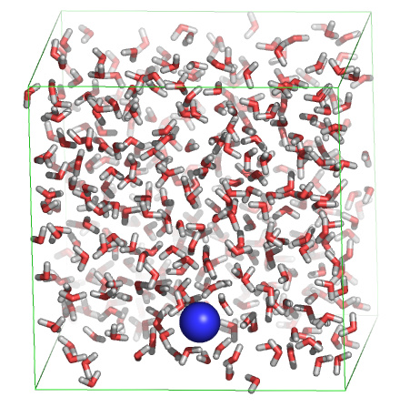
to use this procedure to calculate the free energy of solvation for a
sodium ion in water. For this, we'll slowly create a sodium ion in a
water box. In order to start the simulation, download the
starting coordinates, the
topology, and the MD parameter file first.
We are now going
to use this procedure to calculate the free energy of solvation for a
sodium ion in water. For this, we'll slowly create a sodium ion in a
water box. In order to start the simulation, download the
starting coordinates, the
topology, and the MD parameter file first.
wget http://www3.mpibpc.mpg.de/groups/de_groot/compbio/p8/start.pdb
wget http://www3.mpibpc.mpg.de/groups/de_groot/compbio/p8/na.top
wget http://www3.mpibpc.mpg.de/groups/de_groot/compbio/p8/ti.mdp
pymol start.pdb
gmx grompp -f ti -c start.pdb -p na -maxwarn 2
gmx mdrun -v -c charged.gro
Analyse the free energy change by:
xmgrace dhdl.xvg
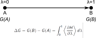
In order to compute the approximate free energy, we must integrate dH/dlambda over
dlambda. Instead, we have dH/dlambda as a function of time. This is
not a problem, as we know that lambda changed from0 to 1 during this
time (10 ps). So instead, we can integrate the curve over time, and
divide the obtained value by ten to derive the desired free energy.
To integrate, under "Data", select "Transformations", followed by
"Integration", and press "Accept".
Question:
The experimentally observed solvation free energies for sodium range
from -365 to -372 kJ/mol. How does the obtained value correspond to
that?
Instead of integrating dH/dlambda, we can also compare the initial and final values of the potential energy of the system:
gmx energy
Select "Potential", followed by "0" (and, if necessary, an extra "enter").
xmgrace energy.xvg
Subtract the initial value from the final value.
Question:
What value do you get? Why is this value different from than the free energy difference obtained by integrating
dH/dlambda?
One important check in simulations in general and in free energy simulations in particular is to make sure that the answer has converged. In order to do so, we can either perform a longer (or shorter!) simulation, and compare the result to the original, or we can perform the backward transition to see if the free energy difference is the opposite of the forward transition. In this practical, we'll do both. First, we'll carry out the backward transition. Copy the MD parameter file to incorporate the changes:
cp ti.mdp back.mdp
and open "back.mdp" in your favorite editor (xedit, nedit, emacs,
kate, vi)
to make the following changes:
First search for "Free energy", then change "init-lambda" to 1 and
change delta-lambda to "-0.0002". Now we can start the backward
simulation. For this, we'll use the final structure of the previous
simulation (charged.gro) as initial structure:
gmx grompp -f back -c charged.gro -p na -maxwarn 2
gmx mdrun -v
And analyse the free energy change using xmgrace. Remember that we now
changed lambda from one to zero, meaning that if we integrate over
time, we should divide the obtained value by -10 instead of by 10.
Question:
What value do you get? How does this value compare to the free energy
change for the forward simulation? Would you consider the obtained
value for the solvation free energy sufficiently converged?
Question:
If we take the forward and backward
simulation together, is the total free energy change positive or
negative? Which of the two should it have been?
As stated above, another way to check convergence is to perform a longer simulation and see if the free energy change remains the same as compared to a shorter simulation. For this, open "ti.mdp" in your favorite editor. Change "nsteps" from 5000 to 50000, and "delta-lambda" from 0.0002 to 0.00002, and repeat the forward transition:
gmx grompp -f ti -c start.pdb -p na -maxwarn 2
gmx mdrun -v
Question: Is the obtained free energy very different as compared to the shorter simulations? What would you consider an appropriate length for this type of simulation?
Go back to Contents
 For the case of a sodium ion in water we could compute the free energy
difference between two states because we defined a path connecting the
two states, and we had access to the free energy gradient along the
path. In the case of the ion in water, the path was an artificial path
(hence such free energy perturbation studies are also called
"computational alchemy"). Likewise, a free energy difference can also
be computed along a real path, e.g. by forcing an ion across an
electrostatic gradient and integrating the force required to displace
the ion along the path.
For the case of a sodium ion in water we could compute the free energy
difference between two states because we defined a path connecting the
two states, and we had access to the free energy gradient along the
path. In the case of the ion in water, the path was an artificial path
(hence such free energy perturbation studies are also called
"computational alchemy"). Likewise, a free energy difference can also
be computed along a real path, e.g. by forcing an ion across an
electrostatic gradient and integrating the force required to displace
the ion along the path.
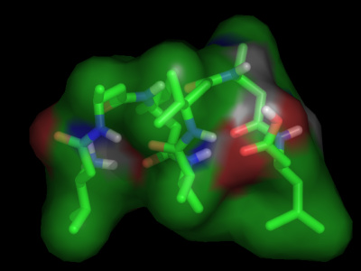
To illustrate the above, we are going to calculate the free energy of
the folding of a small peptide. For this, download a
PDB file of the peptide and the MD trajectories at four different
temperatures: 298K, 340K,
350K and 360K.
wget http://www3.mpibpc.mpg.de/groups/de_groot/compbio/p8/pep.pdb
wget http://www3.mpibpc.mpg.de/groups/de_groot/compbio/p8/298.xtc
wget http://www3.mpibpc.mpg.de/groups/de_groot/compbio/p8/340.xtc
wget http://www3.mpibpc.mpg.de/groups/de_groot/compbio/p8/350.xtc
wget http://www3.mpibpc.mpg.de/groups/de_groot/compbio/p8/360.xtc
First view part of one trajectory with VMD:
gmx trjconv -s pep.pdb -f 340.xtc -o movie.pdb -e 10000 -fit rot+trans
and select "4" followed by "1" when asked to select a group.
vmd movie.pdb
in VMD, play with different representations (under Graphics ->
Representations, e.g. "Licorice") and press the "play" button on the bottom of the main
window. You see the first folding transition during the simulation at
340 K.
Question:
What kind of structure is the folded structure?
For a more quantitative analysis of the folding/unfolding transitions, we'll analyse the root mean square deviation of each structure in each trajectory with respect to the folded structure. Here we will call the structure "folded" if it has a root mean square deviation (RMSD) of less than 2 Angstroms (0.2 nm) of the backbone atoms with respect to the reference structure in pep.pdb.
gmx rms -s pep.pdb -f 340.xtc -o rmsd_340.xvg
when asked for a selection of groups, press "4" (Backbone) and "4" (Backbone) again. View the result with xmgrace:
xmgrace rmsd_340.xvg
Question:
How many folding/unfolding transitions do you observe?
Repeat the same procedure for the other 3 temperatures to generate rmsd_298.xvg, rmsd_350.xvg and rmsd_360.xvg. With a command like the following, we can count how many configuration from each trajectory are "folded" or "unfolded":
cat rmsd_340.xvg | awk 'NR >18 &&$2 < 0.2 {print $0}' | wc -l
if the counting didn't work, then try:
cat rmsd_340.xvg | sed 's/0\./0,/g' | awk ' NR > 18 && $2 < 0.2 {print $0}' | wc -l
(never mind if you didn't understand that command completely. We first throw
away the header of the rmsd_340.xvg file, and afterwards "awk" only prints the lines of which the second column (the RMSD) is smaller
than 0.2; the "wc -l" simply counts the number of lines). The sed command,
finally, replaces the dots in the file with comma's, for the case your
computer expects german input, which uses comma's for floating point numbers.
The obtained number is the number of "folded" configurations in the 340K
simulation. Repeat the procedure, now to count the number of
"unfolded" conformations. You'll see, at this temperature the system
is folded about one third of the time.
You can of course modify and rerun the command manually. The more programming-oriented might however benefit from the following reminder on how to do for loops in bash:
for traj in 298 340 350 360; do;
echo Doing traj $traj   -------------------;
gmx rms -s pep.pdb -f "$traj".xtc -o rmsd_"$traj".xvg;
other command goes here;
done;
Question:
What is the difference in free energy between the folded and unfolded
state at this temperature? (Hint: kT = 2.5 kJ/mol at 300K)
Question:
What about the other three temperatures? What would you estimate to be
the folding temperature?
Question:
Do the above free energy estimates, based on peptide configurations, include
the influence of the solvent? Would different folding free energies (and/or
an estimate of the folding temperature) be obtained when the solvent would be
analysed as well?
Question:
Assuming that the folding enthalpy is the same for the different
temperatures, how can the entropy difference between the folded and
unfolded state be estimated from the set of free energies? How large
do you estimate the entropy of folding in this case? Is it positive or
negative? Why?
Books:
Advanced reading:
Hope you enjoyed it. In case of questions or suggestions, please do not hesitate to contact Bert de Groot: bgroot@gwdg.de