 In the previous lectures we've learned about the theoretical basis of electronic
structure calculations. Here we use a number of methods, and, in
particular, the Hartree-Fock method that is suitable to
compute properties near the ground state of the molecule.
In the previous lectures we've learned about the theoretical basis of electronic
structure calculations. Here we use a number of methods, and, in
particular, the Hartree-Fock method that is suitable to
compute properties near the ground state of the molecule.
In short, the key approximation of Hartree-Fock (HF) is
to model the electron wave function as a single Slater determinant. Recall from the second lecture that
this can only be an approximation because the Slater determinant is an (anti-symmetrized) product of single-electron
wave functions. However, a product of single-electron wave functions would solve the Schrödinger only in case
of non-interacting electrons, which is obviously not exactly correct.
Nevertheless, HF provides a reasonable approximation for the
ground state. In addition, HF is of high interest because it is essentially the starting point of quantum chemistry.
In the context of HF, we here use only the "Restricted Hartree-Fock" (RHF) method, where the orbitals
are double occupied by electrons, that is, we have "closed shell" systems.
Now it is time to jump into the electronic structure business and perform
a couple of calculations by yourself.
The package we are going to use is called GAMESS. There are a number
of GAMESS versions around. GAMESS(US) is free of charge and developed
at Iowa State University. There is also a proprietary version, named
GAMESS(UK), which is developed in England. Finally, a branched program
called PC-GAMESS/Firefly is available. Here, we use
GAMESS(US). Other
popular quantum chemistry packages are Gaussian and Molpro, but they
require a licence.
To start a calculation we basically need four things:
The files needed for this practical can be downloaded as an archive and unpacked by typing
wget http://www3.mpibpc.mpg.de/groups/de_groot/compbio2/p6/praktgamess.tar.gz
tar xzvf praktgamess.tar.gz
cd praktgamess/H2/
The H-H molecule
Our first calculation will be the simple H2 molecule, which is the smallest
molecule that exhibits all fundamental aspects of chemical bonding (why?).
A simple input for the electronic structure calculation of H2 is given
below. In your directory it is called "h2.inp". Have a look at it with your favorite viewer (more, less, emacs,
vi, ...)
 $CONTRL SCFTYP=RHF RUNTYP=ENERGY $END
 $BASIS GBASIS=N31 NGAUSS=6 NDFUNC=1 NPFUNC=1 $END
 $DATA
hydrogen molecule with 6-G31
C1
    H    1  0    0  0
    H    1  0.74 0  0
$END
The $CONTROL specifies the type of wave function and calculation that
should be done. We carry a "self-consistent field" (SCF) calculation,
which means that the program iteratively updates the orbitals until a
certain criterium is reached (see next lecture). The "restricted
Hartree-Fock" (RHF) method is applied to compute the SCF.
RUNTYP=ENERGY means we carry out a single-point calculation, that is
we compute the energy of a single structure and do not scan or optimize the atomic
coordinates.
The $BASIS line defines the (surprise) basis set to be used. Using the
so-called Pople notation, we use the 6-31G** basis. G stands for
"Gaussian", so a GTO basis, which is a sum of orbitals of
 . The other symbols indicated 6 Gaussian functions for the inner
(non-valence) electrons and 4 (3+1) for the valence electrons is
used. This is specified the keywords GBASIS and NGAUSS. Two asterisks **
indicate that polarized orbitals are included in the
basis set. The $DATA
block defines arbitrary line for a Title and a symmetry group
(C1 meaning no symmetry is assumed). Finally, each atom name is
defined followed by the charge of the nucleus, and the x/y/z coordinates.
. The other symbols indicated 6 Gaussian functions for the inner
(non-valence) electrons and 4 (3+1) for the valence electrons is
used. This is specified the keywords GBASIS and NGAUSS. Two asterisks **
indicate that polarized orbitals are included in the
basis set. The $DATA
block defines arbitrary line for a Title and a symmetry group
(C1 meaning no symmetry is assumed). Finally, each atom name is
defined followed by the charge of the nucleus, and the x/y/z coordinates.
Note that each block $CONTROL ... $END, $DATA ... $END, etc. must be
closed with an $END, and that a white space is required before the $
starting a block.
Now we start out first electronic structure calculation by typing
Note: If you want to rerun the same .inp file you must first delete the
file ~/scr/h2.dat.
Have a look at h2.log. In case GAMESS complains about a missing Fortran library (libgfortran.so.3), type
export LD_LIBRARY_PATH=~/Downloads/praktgamess
(This assumes that you unpacked the tar archive under "Downloads" in your home
directory. Please change the path appropriately if you have moved the directory elsewhere. Note that you will need to redefine the LD_LIBRARY_PATH variable for every new terminal shell.)
During the calculation GAMESS writes an output file h2.log that communicates the most
important infos to the user. Please extract the following information:
- number of SCF cycles needed for convergence (check for section "RHF SCF CALCULATION")
- the HF energy (section "ENERGY COMPONENTS").
- the dipole moment (section "ELECTROSTATIC MOMENTS")
In the next step we want to perform the visualization of the bonding and antibonding molecular
orbitals (MO) of the H2 molecule. To view the MOs, we will have to use VMD,
a molecular visualization program for displaying, animating, and
analyzing large biomolecular systems using 3-D graphics and built-in
scripting.
Typing
will load information on the relevant MOs from the existing log
file. In the main VMD window, go to Graphics->Representations. First,
make the atoms visible: Choose Licorice as "Drawing Method" and reduce
the "Bond Radius" to, say, 0.1.
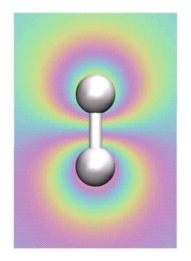
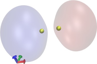 Now let's visualize the orbitals. Select "Create Rep". For the new
representation, select "Drawing Method"->"Orbital", "Coloring
Method"->"ColorID", and "Material"->"Transparent". Now you should see
the lowest-energy MO. Rotate the mouse wheel to zoom out to see the orbital more clearly, if necessary. Also play with the Isovalue. To visualize the
next-lowest MO, create two new representations with the "Create Rep"
button, and select "Orbital"->2 for both of them. Select a positive and
a negative Isovalue for the two representations (e.g., 0.06 and -0.06)
and choose different colors. You should get an image similar to the
one shown here. Browse through the other orbitals and play with the Isovalue.
Now let's visualize the orbitals. Select "Create Rep". For the new
representation, select "Drawing Method"->"Orbital", "Coloring
Method"->"ColorID", and "Material"->"Transparent". Now you should see
the lowest-energy MO. Rotate the mouse wheel to zoom out to see the orbital more clearly, if necessary. Also play with the Isovalue. To visualize the
next-lowest MO, create two new representations with the "Create Rep"
button, and select "Orbital"->2 for both of them. Select a positive and
a negative Isovalue for the two representations (e.g., 0.06 and -0.06)
and choose different colors. You should get an image similar to the
one shown here. Browse through the other orbitals and play with the Isovalue.
Question:
What type of orbitals are the "Orbital" 1, 2, 3, 4, etc.? Compare with
the images in the Wikipedia here and here.
Before continuing, exit VMD.
Go back to Contents
The H-H molecule
potential energy surface
So far, we have only performed so-called single-point calculations, i.e. computed the HF energy
for a fixed nuclear configuration. GAMESS can also scan the energy
along selected coordinates.
In our case of the H2, we will now
determine the energy profile (or the potential energy surface (PES)) along the H-H distance. The input
file "h2scan_rhf.inp" now looks like this:
 $CONTRL SCFTYP=RHF RUNTYP=SURFACE $END
 $BASIS GBASIS=N31 NGAUSS=6 NDFUNC=1 NPFUNC=1 $END
 $SURF ivec1(1)=1,2 igrp1=2 orig1=-0.3 disp1=0.05 ndisp1=150 $END
 $DATA
hydrogen molecule with 6-G31
C1
    H    1  0 0 0
    H    1  0.74 0 0
$END
Note the RUNTYP=SURFACE and the new section $SURF ... $END. The
variables mean that we scan the distance (relative to the initial
distance of 0.74A) between -0.3A and -0.3A + 150*0.05A.
The program will loop over all specified distances and perform for each
of those an independent SCF calculation.
rungms h2scan_rhf.inp >& h2scan_rhf.log
Use the script scanlog2dat.sh
to extract the PES:
chmod +x scanlog2dat.sh
./scanlog2dat.sh h2scan_rhf.log
Have a look at the output file h2scan_rhf_pes.dat with xmgrace.
Question:
Estimate the required energy in kcal/mol to dissociate the H2 (that is, to break
the bond). Note: GAMESS uses the energy unit Hartree (1 Hartree = 627.51
kcal/mol). How does the value compare to the experimental value of 104 kcal/mol?
The HF method gives molecular interaction energies that are only
approximations to the exact quantum many-body energy. In the following we will study the effect
of improving the HF approximation. Here we try
- (a) Configuration interaction (CI). CI is a so-called
Post-Hartree-Fock method that includes correlations between the
electrons (in addition to the exchange energy, which is already
included in HF). During CI, the electronic state is described as a linear
combination of Slater determinants. This is in contrast to HF, which describes the electronic state as
a single Slater determinant;
- (b) Density functional theory (DFT) using the popular B3LYP hybrid
functional. B3LYP stands for "Becke, three-parameter, Lee-Yang-Parr",
who introduced the B3LYP functional.
rungms h2scan_ci.inp >& h2scan_ci.log
rungms h2scan_b3lyp.inp >& h2scan_b3lyp.log
./scanlog2dat.sh h2scan_ci.log
./scanlog2dat.sh h2scan_b3lyp.log
Take a look at all PESs in xmgrace. Hint: use xmgrace -legend load *.dat
Question:
How sensitive is the ground state bond length with respect to the
method? How sensitive is the computed dissociation energy?
Question: Is the bond length
in agreement with the experimental value, which can be found
here. So is the QM level more critical for estimation
of the ground state geometry or to get the dissociation energy right?
Question:
Obviously, Hartree-Fock fails at large H-H distances. What could be an explanation? Hint: Recall that we used the Restricted Hartree-Fock method.

Go back to Contents
The water molecule
Note: if you are running short in time, you could skip this section and proceed with the Caffeine example below.
Let us first switch to the directory where the input for water has been prepared:
Now we are going to move to a slightly more complex molecule having three
nuclei and 10 electrons: the water molecule. We start with an
incorrect geometry of the water molecule and ask GAMESS to optimize
the geometry (note the "RUNTYP=OPTIMIZE" in the input file "water_opt.inp").
During the geometry optimization cycle a SCF calculation
is performed. This one is used to compute the gradient of the total
energy on the nuclei, which is then used
to perform a move of the nuclei. Then the new nuclei positions are
feeded into a new SCF calculation. These
steps are repeated until the structure (=positions of the nuclei) does
not change anymore. As
the basis set, we use the popular 6-31G*, where the * indicates that
d-polarized orbitals on heavy atoms are included (options NDFUNC=1).
 $CONTRL SCFTYP=RHF RUNTYP=OPTIMIZE $END
 $BASIS GBASIS=N31 NGAUSS=6 NDFUNC=1 $END
 $DATA
Water
Cnv 2

  O 8     0  0   0
  H 1    -1  0   0.8
$END
! Meaning that the second H is at +1 / 0 / 0.8
Note that we list only one hydrogen atom here, since the symmetry
group Cnv 2 will generate the second hydrogen.
Run
rungms water_opt.inp >& water_opt.log
and check the output log file with VMD.
In "Graphics"->"Representation" use, e.g., "Drawing Method"->"CPK". Use the
frame bar in the main VMD windows to observe the optimization.
Question:
Which H-O-H angle is predicted? (Check the section "EQUILIBRIUM
GEOMETRY LOCATED" in the log file and calculate the angle from the
coordinates). Hint: you can also use the script log2angle.sh with the log
file as argument:
chmod +x log2angle.sh
./log2angle.sh water_opt.log
Use the simpler
basis set 6-31G by removing the keywords NDFUNC=1 from
water_opt.inp and re-run, after removing the scratch files from the previous run:
\rm ~/scr/water_opt.dat
rungms water_opt.inp >& water_opt.log
./log2angle.sh water_opt.log
Question: Which angle do you now get?
The generated MOs can again be visualized using VMD:
Have a look at all occupied MOs and elucidate their role for bonding in the water monomer.
Which atomic orbitals of the individual atoms are predominately participating in each MO?
Compare the MOs with the ones shown on the following web site:
Molecular Orbitals of the Water Monomer
Question: Where are the
electrons of the 2a1 orbital predominantly located? Hint: play with
the Isosurface.
Go back to Contents
The caffeine molecule
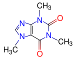
 Finally we are going to compute the electronic structure of the well-known
Caffeine molecule, which is a xanthine alkaloid compound that acts as a stimulant in humans.
The structure of this biomolecule is shown to the left.
Finally we are going to compute the electronic structure of the well-known
Caffeine molecule, which is a xanthine alkaloid compound that acts as a stimulant in humans.
The structure of this biomolecule is shown to the left.
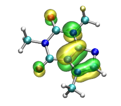
Take a quick look into caffeine.inp. Then type to start the HF calculation,
and visualize the orbitals in VMD
cd ../caffeine
rungms caffeine.inp &> caffeine.log
vmd caffeine.log
Hint: Use two representations, one for the atoms (Drawing Method =
CPK) and one for the orbital, then browse through the orbitals. Use
the buttons "OrbList" and the drop-down list "Orbital" and play with
the Isovalue.
Question: How many orbitals
are occupied? Hint: If you don't like counting try in VMD console: molinfo
top get orboccupancies and molinfo top get numelectrons.
Visualize the so-called HOMO (highest occupied molecular orbital).
Question: How many orbitals
are located around a single atom?