Langevin dynamics
As discussed in the lecture molecules can visit multiple minima between which frequent transitions take place. Modeling the minima as Markov states has proven highly useful not only to map the sometimes complex energy landscapes of biomolecules, but also to comprehensively collect the data from multiple individual runs or to guide future runs by identifying undersampled regions of configuration space.
Today we will focus on the dynamics of a simple system: a single particle in a
box that can diffuse between multiple minima. The advantage of this setup is
that is straightforward to simulate but nevertheless shows interesting dyamics
that resembles some aspects of more complicated (bio)molecular dynamics.
In Langevin dynamics, the force is described by the gradient of the potential,
a friction term and a random term. The latter two terms mimick the dynamic effects of
solvent drag and random solvent kicks. The temperature is controlled by the
strength of the random solvent kicks:

Here M is the mass, X the coordinate, U the potential energy, γ is the friction constant, kB is Boltzmann's constant and R is Gaussian distributed noise.
For this practical, we'll download the archive file "markov.tar.gz" to your current directory and unpack it:
wget http://www3.mpibpc.mpg.de/groups/de_groot/compbio2/p15/markov.tar.gz
tar xvzf markov.tar.gz
cd markov
Please note that the commands in the gray boxes can be easily copy-pasted in the command terminal. Under linux, this is done by selecting the text with the mouse (keeping the left mouse button pressed) and moving to the command terminal and pressing the mouse wheel (middle button) to paste the command. Press ENTER to execute.
Now start the simulation:
./langevin < langevin.inp > langevin.out
This will take a few minutes. In the meantime, please try to answer the following question:
Question:
Once the simulation has finished, the coordinates as a function of time will
be in the trajectory "langevin.out". What analysis could we carry out with the
coordinates to find out if the simulation result can be described as a Markov process?
Go back to Contents
Clustering
Right, let us first have a look at the trajectory:
xmgrace -free -maxpath 1000000 langevin.out
Question:
How would you describe the dynamics? How many clusters can you identify?
In xmgrace, make a histogram of the distribution. Under data, click
transformation, and then histograms. Now Under Source Set, click set 1 (G0) ,
and fill in the starting field (0), stop field (10) and the number of bins
(100), and select "accept". To see the results, double click on one of the
graphs, and click on the first set with the right mouse button, and press
"hide". Now close the window and press autoscale (The "AS" in the top left
under "draw").
Question:
Between which two peaks (minima) would you expect the most frequent
transitions?
For technical reason, we first need to add the following environement variable:
export LD_LIBRARY_PATH=$(pwd)
To help us analyse the results, we are going to use a clustering algorithm and we will try to assign the data to three clusters:
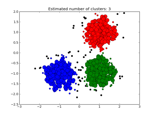
./clus1.csh 1.5
Each cluster is assigned a different color.
Question:
What do you think of the clustering? Could we do better?
Try again, now with a slightly relaxed cutoff for the cluster assignment (2 standard deviations orm each cluster center instead of 1.5):
./clus1.csh 2.0
In fact we have looked at the result in one dimension (the x-coordinate), but the simulation took place in 3D. Have a look at a fragment of the trajectory:
pymol ld.pse
And press the play button.
So let us have a look at the sampled distribution in 3D together with the clustering we had carried out (the green/blue/cyan points are snapshots assigned to different clusters; the data points not allocated to any cluster are colored in red):
./clus2.csh
We can visualize the clustering with PyMol:
pymol cluster.pdb -d "show sphere; spectrum b"
Question:
What do you now think of the clustering?
Obviously, we should use the full dimensionality of the problem for clustering:
./clus3.csh 1.5 1
Again, we use PyMol to visualize the clustering:
pymol cluster.pdb -d "show sphere; spectrum b"
The red points are snapshots that could not be assigned to any cluster. The next step in deciding whether the transitions between the minima (clusters) can be described as a Markov process is to observe the transitions between the clusters:
./trans < cluster.out
This gives us an overview over the transition rates between the clusters.
Question:
Initially, based on the histogram from the 1-dimensional analysis, we had seen
two peaks close to each other (near coordinate positions 2 and 4) and one
further away (near 8). These correspond to clusters 3, 2, and 1,
respectivly. Accordingly, we would expect to see more transitions between
clusters 2 and 3 than between 1 and 2 or between 1 and 3. Why is this not the
case?
Markov state modeling
One of the main characteristics of a Markov process is that it is memory-less. In other words, in a set of Markov states A, B and C, if the system is now in, say, state A, it does not "remember" if it previously came from B or C. Put differently, any transition between states is independent of the history of previously visited states. To evaluate if that is the case for the simulated system, please have a close look at the lower table printed by the program "trans" , entitled "Conditional transition probabilities", that list the transition probabilities between states, keeping track of where the system was before.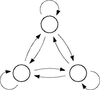
Question:
Is the Markovianity condition of memory-less transitions met? Hint:
transitions such as "1 2 1" and "1 2 3" should have equal conditional
probabilities for a true Markov process.
Possibly, we took too-closely placed snapshots for the clustering, resulting in "memory" for the transitions. Let us try again with more spacing between the snapshots by taking only every 10th snapshot:
./clus3.csh 1.5 10
./trans < cluster.out
Question:
Does the system now behave more Markovian?
The very last line in the output of the "trans" program entitled "mean
deviation from memory-less probabilities" summarizes the differences between
the probabilities that should have been identical in an ideal Markov
process.
Question:
With what spacing between snapshots does the system behave most "Markovian"?
Why does the deviation from an ideal Markov process rise again after first
decreasing with increased spacing?
Another test to assess if the system behaves like a true Markov process is to see if the system's behaviour deviates from a true simulated Markov process based on the same transition rates that we derive from the simulation. Let us test for a spacing of 50:
./clus3.csh 1.5 50
./trans < cluster.out
and now we can simulate an ideal Markov process using the same transition probabilities:
./markov 3 50000 3902809 < markov.inp > markov.out
and analyse the results:
./trans < markov.out
Question:
Does the Langevin simulation result deviate significantly from the true Markov simulation?
As you've seen also the true Markov simulation result deviates from a perfect outcome. Could this be due to a finite simulation length? Let us make the "real" Markov simulation 10 times longer to find out:
./markov 3 500000 3902809 < markov.inp > markov.out
./trans < markov.out
Go back to Contents
Optional: further analysis
- Will memory effects be more or less severe for heavier particles? Test by changing the mass in langevin.inp and rerun the simulation + analysis.
- Will the system behave more like a Markov process or less in a more viscous solvent? Try changing the friction in langevin.inp.
- How will the behaviour change with an increased or decreased temperature?
- Change the position, width, or depth of the energy minima in the landscape. When do you see the largest deviation from ideal Markov behaviour? Why?