

Next: Summary and Discussion
Up: Conformational Dynamics
Previous: A Langevin Model
The question arises, whether memory-effects also show up
at longer time scales, e.g., in the range of few 100 picoseconds.
Viewed at that time scale,
the dynamics of the protein model is characterized
by transitions between the three distinct conformational states
apparent in Fig.  . Accordingly, we shall now neglect the
fast protein dynamics within each conformational substate and
instead focus on the (discrete) conformations dynamics governed
by transitions between the three substates of our model.
To study memory effects at that time scale we will check,
whether the distribution of transition times
between the conformational states can be described by a memory-free
stochastic dynamics,
i.e., we compare the observed conformational dynamics
with the three-state continuous
Markov process depicted in Figure
  .
.
This Markov
process has three states  , which shall represent
the three conformational states defined in Fig.
  and which
are shown together with all possible transitions (arrows)
and corresponding transition rates,
  (
( ).
The probabilities
  to find the model in state
 at time
t
obey the master equation

The time-independent transition rates
 are defined by the conditional probability of
finding the system in state i
at any time t=0, if it has been in state
j before at time
 :
:


Figure: Transition diagram of the three state Markov process used
to describe the transition dynamics of the protein model (see text).
Three states, B,C, and D, corresponding to the three maxima of the
configuration space density projection in Fig.  ,
are connected via conformational transitions (arrows). The stochastic
dynamics of that model is specified by the values of
nine transition rates
  .
.
In order to decide, whether the observed conformational dynamics is
Markovian, we need to check (cf. Ref. Rice65),
whether the probability for a particular transition
depends on the history of the process, i.e., whether
the conditional probabilities listed below are independent of
the time intervals  ,
,
 :
:

Of course, the limited set of available data (a total of
238 conformational transitions) does not allow to verify
all the above conditions. Instead, we restrict our analysis to a comparison
of only the first and second order conditional probabilities,
 and
and
 , respectively.
In addition, we consider only probabilities
 derived from equally spaced instances of time.
In applying this slightly less rigorous test, we assume that
`partial amnesia' is not likely to appear within the dynamical systems
considered here, that is, our analysis does not
apply to processes, which exhibit long-term memory, but at the same time
do not show short-term memory. This assumption is supported
by the results of the preceding section, where it was shown, that the
dynamics of our model does exhibit short-term memory.
Estimates for the first and second order conditional probabilities
 and
and
 were computed from frequency counts derived from the 232 nanoseconds
of simulation data by

Here, the frequency counts  ,
,
 , and
, and
 ,
where
  , are defined in analogy to
(
 ):
):  denotes, how often in the course of the
simulations the model has been found in substate j;
 denotes the number of times
it has been found in substate i, if it has been in substate
j a particular time span
 before, and
 , how often
it has been found in substate i, if it has been in substate
 before and in substate
 ,
,
 before:

The frequency counts were determined using a sample rate of
 .
Here,
  denotes the Kronecker symbol, being unity, if
the protein model is in conformational state
i at time
t, and zero otherwise.
In order to test the hypothesis that corresponding first order and second
order conditional probabilities are equal, in which case the observed
conformational dynamics would be Markovian, the statistical significance
of observed deviations of the probability estimates  from
from
 had to be determined. Accordingly, we
estimated the corresponding standard deviations
  from our
data by

using the Gaussian approximation for binomial probability distributions.
From the set of 27 possible probability distributions  ,
,
 which we examined,
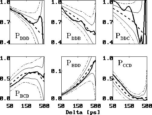
Figure
  shows a selection of six typical cases.
These are the second order conditional probability estimates
 ,
,
 ,
,
 ,
,
 ,
,
 , and
, and
 computed in the range
  ps (bold, solid lines)
which are compared with the corresponding first order conditional
probability estimates,
  (bold, dashed).
Also shown is a
  -interval
(thin, solid) as well as a
  -interval (thin, dashed dotted),
computed according to (
 ).
).
The main observation is that the deviations of the second order
conditional probabilities from
the first order probabilities do not exceed  , i.e.,
with a significance of 2% the data are consistent
with the hypothesis that the conformational dynamics of our model
is indeed Markovian.
This is also true for the remaining
21 probability distributions not shown in Fig.
  .
For a closer analysis we note, that although
the three second order probabilities,
  ,
,
 , and
, and
 (upper half of Fig.
  )
correspond to the same first order probability,
  , the particular
error ranges vary considerably as a result of the different
population densities of the three states.
Whereas the broad error
ranges of
  or
or
 , resulting from a low population
density of state C do not provide much significance, the narrow ranges
apparent for
  or
or
 , resulting from a large number
of transitions between these
highly populated states, provide a good check for non-Markovian
memory-effects. The largest deviation (
 )
was observed for
  in the time range below 60 ps. One may
speculate, that this deviation might
be due to a minor memory-effect present in the rapid decay dynamics
from conformational state C into
D.

Figure: Comparison of six selected second order conditional
probabilities  (bold, solid) with the corresponding first order
conditional probabilities
  (bold, dashed), as described in the text.
The statistical error due to the limited data set is depicted
as a
  -range (thin, solid lines) centered at
 , and
a
  -range (thin, dashed-dotted), respectively.
The above analysis of the distribution of conformational
transition times shows, that
the conformational dynamics of our model is actually well described
by a Markov model suggesting that no memory effects are present
at the corresponding time scale of a few hundred picoseconds.


Next: Summary and Discussion
Up: Conformational Dynamics
Previous: A Langevin Model
Helmut Grubmueller
Mon Nov 6 16:25:56 MET 1995
 . Accordingly, we shall now neglect the
fast protein dynamics within each conformational substate and
instead focus on the (discrete) conformations dynamics governed
by transitions between the three substates of our model.
To study memory effects at that time scale we will check,
whether the distribution of transition times
between the conformational states can be described by a memory-free
stochastic dynamics,
i.e., we compare the observed conformational dynamics
with the three-state continuous
Markov process depicted in Figure
  .
.


 , which shall represent
the three conformational states defined in Fig.
  (
( ).
The probabilities
  to find the model in state
 at time
t
obey the master equation

 are defined by the conditional probability of
finding the system in state i
at any time t=0, if it has been in state
j before at time
 :
:


 .
. ,
,
 :
:

 and
and
 , respectively.
In addition, we consider only probabilities
 derived from equally spaced instances of time.
In applying this slightly less rigorous test, we assume that
`partial amnesia' is not likely to appear within the dynamical systems
considered here, that is, our analysis does not
apply to processes, which exhibit long-term memory, but at the same time
do not show short-term memory. This assumption is supported
by the results of the preceding section, where it was shown, that the
dynamics of our model does exhibit short-term memory.
 and
and
 were computed from frequency counts derived from the 232 nanoseconds
of simulation data by

 ,
,
 , and
, and
 ,
where
  , are defined in analogy to
(
 denotes, how often in the course of the
simulations the model has been found in substate j;
 denotes the number of times
it has been found in substate i, if it has been in substate
j a particular time span
 before, and
 , how often
it has been found in substate i, if it has been in substate
 before and in substate
 ,
,
 before:

 .
Here,
  denotes the Kronecker symbol, being unity, if
the protein model is in conformational state
i at time
t, and zero otherwise.
 from
from
 had to be determined. Accordingly, we
estimated the corresponding standard deviations
  from our
data by

 ,
,
 which we examined,
Figure
  ,
,
 ,
,
 ,
,
 ,
,
 , and
, and
 computed in the range
  ps (bold, solid lines)
which are compared with the corresponding first order conditional
probability estimates,
  (bold, dashed).
Also shown is a
  -interval
(thin, solid) as well as a
  -interval (thin, dashed dotted),
computed according to (
 , i.e.,
with a significance of 2% the data are consistent
with the hypothesis that the conformational dynamics of our model
is indeed Markovian.
This is also true for the remaining
21 probability distributions not shown in Fig.
  ,
,
 , and
, and
 (upper half of Fig.
  , the particular
error ranges vary considerably as a result of the different
population densities of the three states.
Whereas the broad error
ranges of
  or
or
 , resulting from a low population
density of state C do not provide much significance, the narrow ranges
apparent for
  or
or
 , resulting from a large number
of transitions between these
highly populated states, provide a good check for non-Markovian
memory-effects. The largest deviation (
 )
was observed for
  in the time range below 60 ps. One may
speculate, that this deviation might
be due to a minor memory-effect present in the rapid decay dynamics
from conformational state C into
D.

 (bold, solid) with the corresponding first order
conditional probabilities
  (bold, dashed), as described in the text.
The statistical error due to the limited data set is depicted
as a
  -range (thin, solid lines) centered at
 , and
a
  -range (thin, dashed-dotted), respectively.